Blowing pressures in reed woodwind instruments
Leonardo Fuks and Johan Sundberg(1996), KTH TMH-QPSR
3/1996, 41-57, Stockholm, to appear in a revised, modified and improved version as "Blowing pressures in bassoon,
clarinet, oboe and saxophone", in press for Acustica/acta acustica.
Abstract
The blowing pressures during wind instruments playing have not been systematically measured in previous research, leaving the dependencies of pitch and dynamic level as open questions. In the present investigation, we recorded blowing pressures in the mouth cavity of two professional players of each of four reed woodwinds (Bb clarinet, alto saxophone, oboe, bassoon). The players performed three different tasks: (1) a series of isolated tones at four dynamic levels, (2) the same series with a crescendo-diminuendo tones and (3) ascending-descending musical arpeggio played legato at different dynamic levels (pp, mp, mf, ff). The results show that, within instruments, the players pressures exhibit similar dependencies of pitch and dynamic levels. Between instruments, clear differences were found with regard to the dependence on pitch.
Introduction
Blowing pressures in wind instruments, which range between 10 and 120 cm H2O in reed woodwinds, have been a matter of interest in different fields such as respiratory physiology and pathology, occupational health, music acoustics, sound synthesis based on physical models and musical playing practice.
In medical sciences, the information on blowing pressures may be helpful to understand the etiology of some health problems in players and to evaluate the subjects capacity to perform various musical works.
In music acoustics, pressure data are required for comprehension of how the system consisting of player/instrument converts aerodynamic energy into sound. The complex relationship between input parameters (mouth pressure, air flow, and the embouchure, i.e. the constellation of forces and positions in the lip and mouth regions) and the resulting sound properties (pitch variations, loudness and sound quality) represent a challenging and promising issue in the physics of instruments.
For sound synthesis purposes, the input pressure at the instrument is a determinant parameter for sound production and thus required for a successful numerical modelling of the instrument.
In musical practice and education, objective facts regarding playing are valuable for the music teacher/performer and sometimes also for the composer, as such information may have important consequences in playing techniques.
Some earlier investigations have included data on blowing pressures in wind instruments. Bouhuys (1968) studied the oboe and clarinet and other instruments and presented pressure ranges for low and high tones. Navrátil & Rejsek (1968) observed that blowing pressures varied with dynamic level in clarinet, oboe and bassoon. Worman (1971) describes the behaviour of a clarinet in terms of the relation between flow velocity and blowing pressure but does not present any information on the dependence of pressure on dynamic level. Pawlovski & Zoltowski (1985) give some general pressure ranges for bassoon and clarinet, obtained from a numerous set of subjects, including students and professionals. Pawlovski & Zoltowski (1987) provided more specific results for two notes and two dynamic levels in clarinet, oboe and bassoon. Their main aim was to formulate a distinction between normal and pathologically reduced maximum playing duration for a tone. Fuks (1993) measured blowing pressures in clarinet at three dynamic levels, pitches G3, F4 and E5, played by only one subject using four different reeds.
Summarizing, the data available on blowing pressures in wind instruments are scarce, particularly with respect to dependence on pitch and dynamic levels and confined to sustained tones, lacking a musical context. The purpose of the present investigation was to measure blowing pressures in wind instrument players at four different dynamic levels and at pitches covering the normal range of the instruments. For the sake of limitation, the investigation was confined to four reed instruments, clarinet, alto saxophone, oboe and bassoon.
Material and method
Mouth pressure was captured by means of a thin pressure transducer (Gaeltec 7Sb) inserted in the players mouth corner, so as to minimally affect the embouchure. The transducer was connected to an amplifier and one track of a multichannel TEAC (RD-200T) PCM DATA recorder. A sound level meter (Ono Sokki LA-210) and a microphone (Sony ECM-959DT), both at 1 m distance, picked up the audio signal and its SPL. The signals from both these devices were recorded on separate tracks of the same TEAC recorder. Experiments were run in a moderately reverberant room, volume close to 70 m3 (615 x 460 x 250 cm).
The experimental protocol consisted of the following tasks:
1. Sustained tones (Table 1) in a series of ascending fifths, played four times at each of four different dynamic levels forte, f, pianissimo, pp, mezzopiano, mp, and mezzoforte, mf, duration of about 2 seconds each. This task was performed 3 times. These data will be referred to as fs , mfs , mps and pps .
2. The same sequence of pitches as in the previous item, in ascending and descending order, played crescendo-diminuendo from pp to mf to pp. Each tone had a duration of 3 seconds, approximately. This series was played three times. As expected, a pressure variation was observed during the tones, as illustrated in Figure 3. Therefore three pressures were measured for each tone, at the onset, at peak and at the termination. These pressures will be referred to as bo , bp and bt.
3. Ascending and descending arpeggi (see table 1), tones of 1s duration, approximately, covering the typical pitch range of the instrument. These arpeggi were played legato at four dynamic levels (fortissimo, ff, pianissimo, pp, mezzopiano, mp, and mezzoforte, mf). Each level was played four times in succession. Henceforth, the data from this task will be referred to as ffa , ppa , mpa and mfa.
One of the pitches played in these tasks was common (marked with bold characters in Table 1). As can be seen in the table, this tone was located in the middle range of the instrument.
For all tasks, subjects were instructed to play as uniformly as possible with respect to tempo, sound quality and loudness. In task 3, the players were instructed that ff and pp referred to the maximum and minimum possible loudnesses that could be produced, keeping acceptable tone quality. The intermediate dynamic levels (mf and mp), were left to the musician to decide. They were also asked to avoid vibrato, as it might be associated with a modulation of the blowing pressure.
Players were aware only of the fact that the experiment was related to blowing pressures and that it would take from 40 to 50 minutes. No other information was given until the entire recording protocol was completed.
Calibration
Table 1. Tones used for the various tasks for the different instruments. Bold characters represent pitches common to all three procedures.
A4= 442 Hz
| Instrument | Series of Fifths - tasks 1 & 2 |
Arpeggio - task 3 |
| Bb Clarinet * | F3 C4 G4 D5 A5 E6 | Eb3 G3 Bb3 Eb4 G4 Bb4 Eb5 G5 Bb5 Eb6 |
| AltoSax (Eb) * | F3 C4 G4 D5 A5 | Eb3 G3 Bb3 Eb4 G4 Bb4 Eb5 G5 |
| Oboe | C4 G4 D5 A5 E6 | Bb3 D4 F4 Bb4 D5 F5 Bb5 D66 |
| Bassoon | C2 G2 D3 A3 E4 B4 | Bb1 D2 F2 Bb2 D3 F3 Bb3 D64 F4 Bb4 |
* refers to actual pitches rather than transposed notations
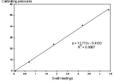
The Gaeltec output voltage was set to zero for ambient air pressure and for every experimental session the range knob was adjusted so as to accommodate the maximum pressures used by the player. After each experimental session, the transducer was immersed at various depths in a water column the lengths of which were measured and the associated output voltages were recorded. The precalibrated sound pressure level meter was exposed to two different SPL values (B&K Calibrator 4230) as references and the output voltages were recorded on the tape. All these calibration signals were also announced on the audio track of the tape. The relation between the Gaeltec output voltage to pressure was found to be linear, the errors being smaller than 1 cm of H2O within the pressure ranges used; a typical example can be seen in Figure 1. Hence, the conversion from voltage to pressure was determined by means of a linear regression trendline applied to the calibration data.
Subjects and instruments
The subjects, two oboists, two bassoonists, two clarinettists and two saxophonists, were all professionals, and represented the western classical music tradition. All subjects had at least 15 years of experience of playing in symphony orchestras. Only one of them was female (clarinettist Cl1). The age range was 32 to 54 years. The musicians played on their own instruments and mouthpieces/reeds, that they used as their everyday working tools. Appendix B specifies the instruments used. As payment for their participation they received an amount approximately corresponding to a one-hour private lesson.
Analysis
The recorded signals were transferred from the Teac recorder into computer files, using the Swell DSP software package installed in a PC computer and an Ariel DSP-16 board.
Mouth pressure voltage was determined for each tone and exported to an Excel spread sheet. For each tone played at constant loudness, mouth pressures were averaged across the quasi-stationary part of the tone. Even for such tones the pressure curves rarely presented a perfect plateau-like shape. In such cases, representative values were determined by eye, with the aid of visual display and zooming, and also of audio playback from the data files. Figures 1, 2 and 3 show typical examples from sustained, crescendo and arpeggio tones. The mouth pressure voltages thus determined were then converted into pressure units.
Figure 1. A typical pressure calibration curve. The transducer was dipped into water at depths of 55, 41, 24, 8 and 0 centimeters. The ordinate corresponds to values read at the Swell software files. The trendline was drawn by Excel which also calculated the line

Figure 2. Sound wave and pressure curves from player Cl2 obtained from Task1 (sustained tones). The horizontal lines show the mouth pressure values selected for analysis.
Figure 3. Sound wave and pressure curves from player Ob1 obtained from two takes of a tone played in Task2 (crescendo-diminuendo). The three horizontal lines show mouth pressures at onset, peak and termination.
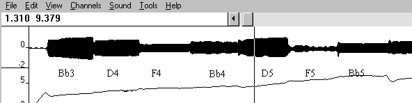
Figure 4. Sound wave and pressure signals as displayed by the Swell software. The pitch names are given below the corresponding tone segment.
For each pitch, mean values were computed across all takes and the standard deviations determined. In cases of four replications, these mean values ± one standard deviation represent a confidence interval of 95%, provided that a normal distribution of the data is assumed.
Results
In this section some examples of micro-structural features of pressure curves will be shown first. Then, the results will be presented instrument by instrument. For each instrument mean pressures measured during the sustained tones and for the crescendo-diminuendo tasks will be presented in terms of histograms. These data show the pressures used under quasi-neutral conditions. It is interesting to compare them with those observed in a musical context such as the arpeggio task. These values are displayed in sets of graphs where the abscissa represents the tones position in the musical score. Averages and standard deviations are listed in tables in the Appendix A. Instruments are specified in Table B, Appendix.
Some micro-structural features of pressure curves
A set of characteristic pressure patterns were observed in the data. Although a detailed examination of them is beyond the scope of this study, they seem to deserve some comments, as they would illustrate the musicians' modus facendi.
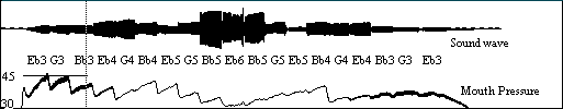
Figure 5. Pressure variations in Player Cl2 mf arpeggio, take 2, illustrating the rising/falling pitch contour effect.
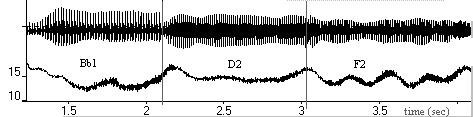
Figure 6. Examples of sound wave and mouth pressure modulation (upper and lower curves) during vibrato in the bassoon observed for notes B1 , D2 and F2 in the arpeggio task played in pp. Pressures in cm of H20.
Rising/falling pitch contour
In the arpeggio task some players increased pressure during each tone in the ascending part but not so in the descending part, as can be seen in Figure 5.
Vibrato
Although the players were instructed to avoid vibrato, some cases of inadvertent vibrato occurred. Figure 6 illustrates an example from the arpeggio task in pp played on the bassoon. A clear pressure modulation can be observed with an amplitude ranging from 1.5 to 3 cm H2O. The frequency and phase of the modulation agree with the amplitude modulation.
Pre-tone pressure build up
Before the tone onset a pressure build-up phase was frequently noted that was followed by a pressure drop after
the onset, which ended on the pressure used for the quasi-stationary remainder of the tone. Figures 7 and 8 show
examples from sustained tones played on clarinet and oboe. Typically the duration of these pressure patterns ranged
from 0.35 to 0.60 seconds, and in the case of the oboe, the amplitude of the peak, i.e. the difference between
the peak and the subsequent quasi-steady pressure, ranged from 3.0 and 7.0 cm H2O, at G4
in mf. This phenomenon could reflect strategies needed for starting well-controlled reed vibrations.
Figure 7. Pre-tone pressure build-up, Ob2, G4, mf Figure 8. Pre-tone pressure build-up, Cl2,
C4, mf
Figure 9. Pressure anticipating clarinet tone, Eb6,
mp, player Cl2. Sound wave and mouth pressures
are displayed in upper and lower curves. Pressures
in cm of H20.
Strategies for producing difficult tones
Tones at pitch extremes are generally more difficult to play than other tones. In some cases, the players established a pressure supposedly suitable for the intended tone which, however, started somewhat later. Figure 9 shows an example from the clarinet.
Clarinet
Figures 10 to 15 present results obtained from the two clarinet players. In general, the data are quite systematic and reasonably similar for both players, and as can be seen in Tables A1 and A2 in the Appendix, the standard deviations for the pp-mp-mf indicate a very consistent behavior of the players. Also, the bo pressures observed at the start of the crescendo-diminuendo tones were very similar to the pps values from the sustained tones, see Figures 10 and 11 from player Cl1. The bp pressures at the peak of the crescendo tones are generally close to the mfs or fs values of the sustained tones. The termination pressures bt of the crescendo-diminuendo tones are in most cases slightly lower than the bo at the onset. The pressure ranges from 20 to 55 cm H2O, and player Cl1 tended to use slightly lower pressures than player Cl2. The loudness increases between the dynamic levels pp, mp and mf correspond to pressure increments. For player Cl1, they range from 3 to 9 cm H2O for the pp, mp, and mf levels, while for the ff level it was up to 15 cm H2O. Player Cl2 used more even steps, ranging from 3 to 9 cm H2O.
The blowing pressures measured in the sustained tones agree reasonably well with those observed in the ascending arpeggio, the maximum discrepancy being up to 3.0 cm H2O in pp , mp and mf. In ff larger differences were observed. Also, both subjects played sustained tones with pressures quite similar to those they used for the neighbouring tones in the arpeggio tasks. There was a quite close agreement between the lowest pressures used for G4, the common pitch to all three tasks. Thus, the pp pressure used in the arpeggio (ppa) was quite similar to the bo in the crescendo-diminuendo tones and also to the ps in the sustained tones.
Another interesting striking characteristic is the fact that the pressure curve in Figures 14 and 15 exhibit a maximum for all dynamic levels of the arpeggio, located at Bb4. This is probably dependent on the fact that this is the point along the pitch scale where overblowing starts. Thus, the fingering for Bb4 is identical to that for the lowest pitch Eb3, except for the opening of the twelfth-key, which produces the overblowing effect.
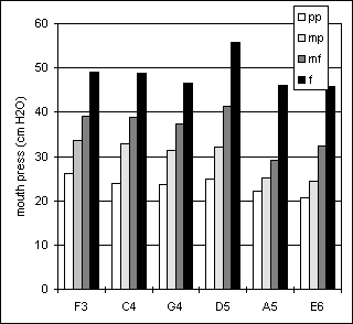

Figure 10. Sustained tones, player Cl1 Figure 11. Crescendo-diminuendo, player Cl1
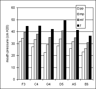

Figure 12. Sustained tones, player Cl2 Figure 13. Crescendo-diminuendo, player Cl2
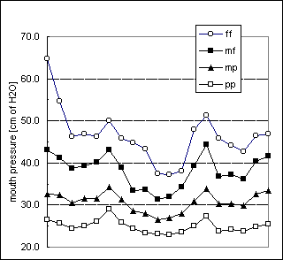
Figure 14. Arpeggio task , player Cl1.
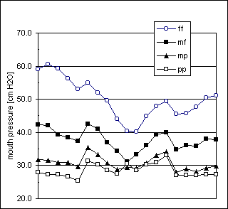
Figure 15. Arpeggio task, player Cl2.
Saxophone
Figures 16 to 21 present results obtained from the two saxophone players. The low standard deviations in the arpeggio task indicate a good intra-subject consistency, see Tables A3 and A4 in the Appendix. For player Sx1, the pressure ranged from 15 to 80 cm H2O, approximately. The highest pressure used by player Sx2 was 55 cm H2O. In general, blowing pressures at low dynamic levels are very close between both players.
As shown in Figures 20 and 21, both players increased pressures when they shifted to a louder dynamic level, except for the lowest pitch, F3. Player Sx1 regarded the pitches Eb3 and F3 as rare tones in symphonic saxophone repertoire; these tones would require a different reed, particularly for soft dynamic levels. This may explain, at least partially, the relatively high pressures for the pitch F3.
The pressures for Sx1s sustained tones do not agree well with those observed in the arpeggio task. However, listening to the recordings and inspecting the SPL values revealed that the sustained tones were played louder than the arpeggio tones.
The pressures used for mfs, sustained tones, agreed closely with the bp values for all tested tones as played by player Sx2, see figures 18 and 19. Pressure steps between sustained tones played at adjacent dynamic levels are also very regular, ranging approximately from 4.0 to 6.0 cm H2O.
Comparing the two players, Sx1 tended to use higher pressures in all tasks.
Combining the data from the three tasks from both players, the blowing pressures seem to slightly increase with pitch in the lowest octave of the instrument, reaching a peak in the region between Eb4 and G4, and decreasing with pitch above this pitch region. It may be relevant that in the alto saxophone overblowing starts in this pitch range, viz. at F4.
Oboe
In all tasks, player Ob 2 tended to use considerably higher pressures than player Ob1, particularly at high pitches and high dynamic levels, see Figures 22 to 27. For Ob1 and Ob2, the pressures ranged from 35 to 95 cm H2O and from 41 to 124 cm H2O, respectively. In both players, the pressures increased not only with loudness but also with pitch, although the pressure range used by player Ob2 is considerably wider than that used by player Ob1.
In both subjects, the values used for the sustained tones agree quite well with those observed both in the crescendo-diminuendo and arpeggio tasks. For both players, the onset pressures, bo, in the crescendo-diminuendo task were very close to the pps values in the sustained tones, see Figures 22-23 and 24-25. Also, the bp pressures in the crescendo tones were generally close to the mfs values while the termination pressures bt were mostly somewhat lower than the bo. There was a quite close agreement between the lowest pressures used for D5, the pitch common to all three tasks, but the pressure steps between dynamic levels were usually smaller in the arpeggio task than in the sustained tones.
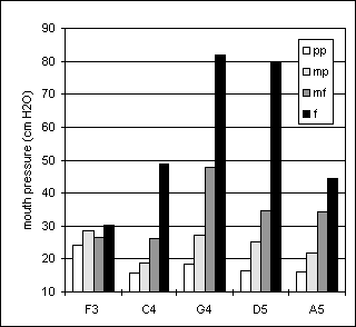

Figure 16 Sustained tones, player Sx1 Figure 17. Crescendo-diminuendo, player Sx1
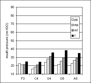
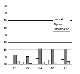
Figure 18. Sustained tones, player Sx2 Figure 19. Crescendo-diminuendo, player Sx2

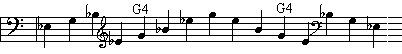
Figure 20. Arpeggio task , player Sx1
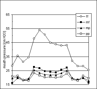
Figure 21. Arpeggio task, player Sx2.

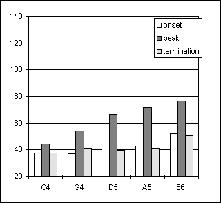
Figure 22. Sustained tones, player Ob1 Figure 23. Crescendo-diminuendo, player Ob1
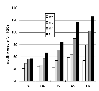
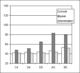
Figure 24. Sustained tones, player Ob2 Figure 25. Crescendo-diminuendo, Player Ob2
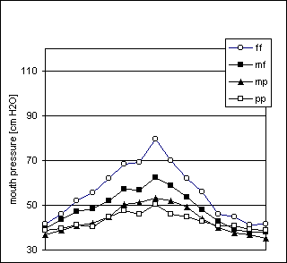

Figure. 26. Arpeggio task, player Ob1
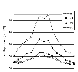
Figure 27. Arpeggio task, player Ob2
In the arpeggio task the pressures used for pp and mp were rather similar, especially for the five lowest tones, as seen in Figures 26 and 27. This suggests that at low dynamic levels, the loudness control is mainly realized with other factors than pressure, such as the embouchure. In both subjects, the pressures used for pp at the lowest pitches are slightly higher than the ones used for mp. The lowest tones of the oboe are particularly difficult to start.
As opposed to the clarinet and the saxophone, the changing of register and the presence of the overblowing effect did not correspond to peaks in the pressure curves.
Bassoon
Figures 28 to 33 present data from the two bassoon players. For players Bn1 and Bn2, the pressure ranged from 12 to 90 cm H2O and from 13 to 52 cm H2O, respectively. Tables A7 and A8 (Appendix) show that Bn1s standard deviations mostly ranged from 1 to 3 cm H2O in pp-mp-mf while player Bn2 presents similar ranges for pp-mp but at mf the standard deviations range from 1 to 5 cm H2O. Still, all takes from each player sounded musically quite acceptable. Pressure increased continuously with both loudness and pitch. As shown in Figures 28 and 30, the pressure steps between adjacent dynamic levels showed some variation in the sustained tones.
In the arpeggio, pressures for pp and mp were rather similar throughout the pitch range, see Figures 32 and 33, while slightly higher pressures were sometimes used for pp than for mp.
Looking at sustained tones and crescendo-diminuendo tasks from both players, Figures 28-29 and 30-31, the bo pressures observed at the start of the crescendo-diminuendo tones are very similar to the pps values from the sustained tones. In a similar way, the bp pressures at the peak of the crescendo tones are generally close to the mfs or fs values of the sustained tones. The termination pressures bt of the crescendo-diminuendo tones are in general lower than the bo at the onset, in a fashion that the difference between bo and bt clearly increases with pitch.
At dynamic levels above pp both subjects played sustained tones with pressures systematically higher than those used for neighbouring tones in the arpeggio. Similarly, pressures used by both subjects for D3, the pitch common to all three tasks, differed between the arpeggio, a musical context, and the sustained tones, a musically more neutral context. On the other hand, the pp pressures in the arpeggio (ppa) were quite similar to the bo in the crescendo-diminuendo tones and also to the ps in the sustained tones.
As with the oboe, no peculiar characteristic was found relative to the overblowing phenomenon.
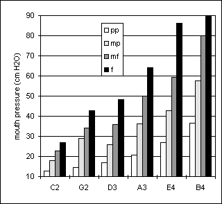
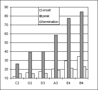
Figure 28. Sustained tones, player Bn1 Figure 29. Crescendo-diminuendo, player Bn1
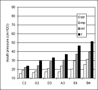
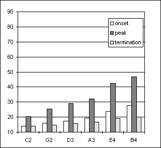
Figure 30. Sustained tones, player Bn2 Figure 31. Crescendo-diminuendo, player Bn 2
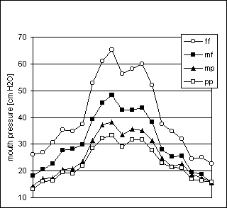
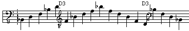
Figure 32. Arpeggio task, player Bn1
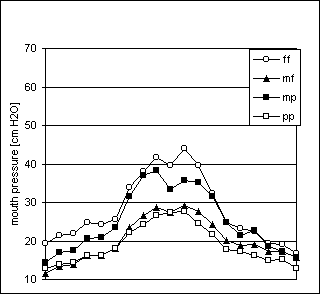
Figure 33. Arpeggio task, player Bn2
Discussion
The present investigation was limited to the blowing pressures. These pressures represent a rather special aspect of the overall blowing mechanism. The air flow through the reed and the embouchure conditions are other important aspects, which, however, we will plan to consider in future investigations. The blowing pressures are important to the understanding of the players work and the instrument behaviour. The air flow is a consequence of the blowing pressure and the resistance offered by the vibrating reed and by the acoustic properties of the air column. The reed system, in turn, is characterized by the geometry and physical properties of the reed, the mouthpiece design and the embouchure.
The data partly agree with those previously reported in the litterature. The pressure ranges observed by Bouhuys (1968) at "low tones" in oboe and clarinet are in reasonable agreement with our results, while his values for "high tones" are clearly higher than those we observed. The pressure ranges for bassoon and clarinet reported by Pawlovski (1985) for numerous subjects (students and professionals) are in reasonable agreement with ours for the clarinet but for the bassoon we observed clearly lower pressures at low pitches. Pawlovski & Zoltowski's (1987) pressure values for identifying good clarinet, oboe and bassoon players do not match our results, which are sometimes much higher and sometimes much lower. On the other hand, our data are in good agreement with the results reported by Fuks (1993) for different loudnesses and pitches played on different reeds by one single professional subject, particularly for the high quality reeds. The systematic dependence on pitch and dynamic level found for the oboe and the bassoon is quite similar to that previously found in singers (Leanderson & al, 1987), although the pressures used in the instrument are obviously much higher.
We tested only two players for each instrument. Mostly both players pressure data exhibited similar pitch and loudness dependences, but in some cases, noticeably in the oboe and the bassoon, one player tended to consistently use higher pressures than the other. These interindividual differences may be due to different reed properties and/or different blowing techniques and personal preferences.
Clarinets on the one hand and the double reeds oboe and bassoon on the other, showed clearly contrasting features as illustrated particularly by the arpeggio curves. In the double reed instruments, pressure tends to be increased continuously with pitch. In the clarinet, pressure tended to decrease with pitch but peaked at the lowest overblowing pitch. These pressure characteristics would be due to the acoustical properties of these instruments, that respond differently depending on their input impedance curves and the reed-instrument interaction. Interestingly, the pressure curves in the lowest octave of the saxophone showed a pattern similar to that of the double reed instruments. However, at higher pitches, where the tones are produced by overblowing, the curves were more similar to those of a clarinet. The saxophone has a conical bore like oboe and bassoon whilst the reed and mouthpiece are similar to those of the clarinet.
In the arpeggi, the pressure curves differed between the ascending and descending parts. Generally, higher pressures were used for the ascending part, particularly at the highest dynamic levels. Probably the reason for this was musical; the players tended to make a crescendo during the ascending part and a diminuendo during the descending part.
The occurrence of higher standard deviations at the ff arpeggio in data from most of the subjects may be due to different reasons. One is that playing as loud as possible is an unrealistic task for symphony orchestra musicians, and hence the players would be unfamiliar with such a task.
Both the experimental protocol and the equipment appeared appropriate for our purposes. Ideally, the blowing pressures should be measured for the entire range of the instrument, but this would increase the length of the recording session beyond acceptability. Keeping the pressure transducer in the mouth corner seemed to inflict marginally on the playing.
The refined use of lung pressure in our players raises the question as to the underlying control system. Mechanoreceptors in the subglottal mucosa have been assumed to play an important role in the control of subglottal pressure during phonation (Wyke, 1976). Poor support for this assumption was found in the case of singing (Sundberg et al., 1995). Still, the mechanoreceptors in the subglottal mucosa might play a more prominent role in the control of the considerably higher blowing pressures in wind instruments. There might also be a strong participation of the whole proprioceptive respiratory system, including abdominal, thoracic and lung receptors, on wind instrument players blowing control that deserves an investigation in the realm of respiratory psychophysics (Katz-Salamon, 1983).
Conclusions
Blowing pressures represent a rather special aspect of the overall blowing mechanism, to which the air flow and embouchure conditions should be added. However, the pressure reflect many aspects of the players work and the instrument behaviour. Our data have revealed characteristic dependences of the pressure on pitch and on dynamic level in clarinet, saxophone, oboe and basson. For each of these instruments, these dependencies seemed consistent within as well as between players, although some players tended to use higher pressures than others. In the double reed instruments, oboe and bassoon, pressure tends to be increased continuously with pitch. In the clarinet, pressure tended to decrease with pitch, but overblowing was produced with higher pressures than the corresponding lower tones. The pressure curves in the lowest octave of the saxophone showed a pattern similar to that of the double reed instruments. However, at higher pitches, where the tones are produced by overblowing, the curves were more similar to those of a clarinet.
Acknowledgements
This study is supported by the Brazilian Ministry of Education (CAPES Foundation), through a PhD scholarship and a research grant, and by the KTH (Royal Institute of Technology), Department of Speech, Music and Hearing. Co-author LFs staying at the KTH was made possible thanks to the Universidade Federal do Rio the Janeiro, School of Music, Department IV. The authors are indebted to the kind cooperation of the players.
References
Backus J (1963). Small-vibration theory of the clarinet. JASA 35: 305-312, p312.
Benade A (1976). Fundamentals of Musical Acoustics. NY: Oxford University Press, 437.
Bouhuys A (1964). Lung volumes and breathing patterns in wind instrument players. Journal of Applied Physiology 19(5): 967-975.
Bouhuys A (1968). Pressure-flow events during wind instrument playing. Sound Production in Man, Annals of the New York Academy of Sciences, Vol. 155, Art.1: 264-275.
Burghauser J & Spelda A (1971). Akustische Grundlagen des Orchestrierens. Regensburg: Gustav Bosse Verlag.
Cossette I (1993). Étude de la Mécanique Respiratoire ches le Flûtistes, PhD Thesis, Université de Montreal.
Fuks L (1993). The sounding bamboo: a study on the quality of clarinet reeds. Production Engineering M.Sc. thesis, written in Portuguese, COPPE/UFRJ, Rio de Janeiro.
Katz-Salamon M (1983). Judgement of Different Ventilatory Parameters by Healthy Human Subjects - A psychophysical study, PhD Thesis, Karolinska Institutet, Stockholm.
Leanderson R, Sundberg J & von Euler C (1987). Role of diaphragmatic activity during singing: a study of transdiaphragmatic pressure. J Applied Physiology 62: 259-270.
Navrátil M & Rejsek K (1968). Lung function in wind instrument players and glassblowers. Sound Production in Man, Annals of the New York Academy of Sciences, Vol. 155, Art.1: 276-283.
Pawlowski S & Zoltowski M (1985). Chosen problems of the aerodynamics of playing the wind instruments. Archives of Acoustics (Poland). 1073: 215-228
Pawlowski S & Zoltowski M (1987). A physiological evaluation of the efficiency of playing the wind instruments - an aerodynamic study. Archives of Acoustics (Poland). 12/3-4: 291-299
Rossing T (1982). The Science of Sound, Addison-Wesley Publishing Co.Reading, Mass.
Sommerfeldt S & Strong W (1988). Simulation of a player-clarinet system. JASA 83(5).
Stewart S & Strong W (1980). Functional model of a simplified clarinet. JASA 68(1).
Sundberg J, Iwarsson J, Bilström A-M H0(1995). Significance of mechanoreceptors in the subglottal mucosa for subglottal pressure control in singers. Journal of Voice, 9/1: 20-26.
Worman W (1971). Self-Sustained Nonlinear Oscillations of Medium Amplitude in Clarinet-Like Systems, PhD Thesis, Case Western Reserve University.
Wyke B & Kirschner J (1976). Neurology of Larynx. In: Hinchcliffe R & Herrison D, eds. Scientific foundation of otolaryngology. William Heinemann Medical Books, 546-566.
Appendix
A. Mouth pressure data tables from arpeggio task
Table A1. Mean and standard deviations of mouth pressures in cm of water, player Cl1
Eb3 |
G3 |
Bb3 |
Eb4 |
G4 |
Bb4 |
Eb5 |
G5 |
Bb5 |
Eb6 |
Bb5 |
G5 |
Eb5 |
Bb4 |
G4 |
Eb4 |
Bb3 |
G3 |
Eb3 |
||
ff |
mean |
65 |
55 |
46 |
47 |
46 |
50 |
46 |
45 |
43 |
37 |
37 |
38 |
48 |
51 |
46 |
44 |
43 |
46 |
47 |
| stdev |
4.5 |
3.7 |
3.3 |
2.3 |
2.4 |
1.9 |
2.0 |
4.1 |
2.2 |
4.4 |
1.3 |
2.9 |
3.0 |
4.5 |
4.9 |
2.9 |
2.9 |
2.9 |
6.3 |
|
mf |
mean |
43 |
41 |
39 |
39 |
40 |
43 |
39 |
33 |
34 |
31 |
32 |
34 |
39 |
44 |
37 |
37 |
36 |
40 |
42 |
| stdev |
2.6 |
0.8 |
1.2 |
0.9 |
1.7 |
2.6 |
2.3 |
1.8 |
1.6 |
3.0 |
1.2 |
2.0 |
0.5 |
3.3 |
2.0 |
1.0 |
1.1 |
2.0 |
1.7 |
|
mp |
mean |
33 |
32 |
30 |
32 |
32 |
34 |
31 |
29 |
28 |
26 |
27 |
28 |
31 |
34 |
30 |
30 |
30 |
33 |
33 |
| stdev |
1.7 |
1.2 |
0.9 |
0.4 |
1.1 |
0.7 |
0.5 |
0.8 |
0.9 |
1.0 |
0.8 |
0.6 |
0.7 |
0.7 |
0.2 |
0.5 |
0.6 |
1.0 |
1.5 |
|
pp |
mean |
26 |
26 |
24 |
25 |
26 |
29 |
26 |
24 |
23 |
23 |
23 |
24 |
25 |
27 |
24 |
24 |
24 |
25 |
26 |
| stdev |
1.0 |
1.4 |
1.3 |
1.4 |
1.2 |
1.6 |
1.2 |
1.0 |
0.8 |
0.5 |
0.8 |
0.9 |
0.8 |
1.0 |
0.9 |
0.3 |
0.7 |
0.4 |
0.5 |
Table A2. Mean and standard deviations of mouth pressures in cm of water, player Cl2
Eb3 |
G3 |
Bb3 |
Eb4 |
G4 |
Bb4 |
Eb5 |
G5 |
Bb5 |
Eb6 |
Bb5 |
G5 |
Eb5 |
Bb4 |
G4 |
Eb4 |
Bb3 |
G3 |
Eb3 |
||
ff |
mean |
59 |
60 |
59 |
56 |
53 |
55 |
52 |
50 |
44 |
40 |
40 |
45 |
48 |
49 |
46 |
46 |
48 |
50 |
51 |
| stdev |
0.7 |
3.8 |
4.1 |
3.0 |
2.7 |
3.9 |
3.3 |
0.7 |
1.1 |
2.5 |
1.4 |
2.8 |
2.2 |
2.1 |
1.8 |
1.9 |
4.8 |
3.6 |
1.2 |
|
mf |
mean |
42 |
42 |
39 |
38 |
37 |
43 |
41 |
37 |
34 |
31 |
33 |
36 |
39 |
40 |
35 |
36 |
36 |
38 |
38 |
| stdev |
1.0 |
1.6 |
2.1 |
2.0 |
1.9 |
2.3 |
1.5 |
1.4 |
1.6 |
1.4 |
0.7 |
1.0 |
1.5 |
0.6 |
1.3 |
1.2 |
1.2 |
2.0 |
2.9 |
|
mp |
mean |
32 |
32 |
31 |
31 |
30 |
35 |
33 |
31 |
29 |
29 |
29 |
31 |
33 |
34 |
28 |
29 |
28 |
29 |
30 |
| stdev |
2.2 |
2.8 |
1.8 |
0.8 |
0.7 |
0.3 |
0.8 |
0.8 |
0.5 |
1.5 |
0.6 |
0.3 |
0.6 |
0.7 |
0.3 |
0.3 |
1.1 |
1.1 |
1.9 |
|
pp |
mean |
28 |
27 |
27 |
27 |
25 |
31 |
30 |
29 |
27 |
31 |
29 |
30 |
31 |
33 |
27 |
27 |
27 |
27 |
27 |
| stdev |
1.3 |
1.6 |
1.7 |
0.8 |
0.7 |
0.5 |
0.7 |
0.4 |
0.7 |
0.5 |
0.8 |
1.0 |
0.4 |
0.9 |
0.5 |
0.9 |
0.7 |
0.6 |
0.6 |
Table A3. Mean and standard deviations of mouth pressures in cm of water, player Sx1
Eb3 |
G3 |
Bb3 |
Eb4 |
G4 |
Bb4 |
Eb5 |
G5 |
Eb5 |
Bb4 |
G4 |
Eb4 |
Bb3 |
G3 |
Eb3 |
||
ff |
mean |
25 |
37 |
43 |
45 |
61 |
60 |
49 |
43 |
45 |
48 |
55 |
35 |
34 |
37 |
26 |
| st.dev. |
1.2 |
3.5 |
4.6 |
1.9 |
4.7 |
5.0 |
4.2 |
5.4 |
4.2 |
2.5 |
4.5 |
2.4 |
5.3 |
2.6 |
1.3 |
|
mf |
mean |
21 |
24 |
28 |
29 |
40 |
39 |
32 |
29 |
32 |
32 |
35 |
26 |
24 |
25 |
21 |
| st.dev. |
0.6 |
1.4 |
2.1 |
1.2 |
1.6 |
1.8 |
2.6 |
1.7 |
2.8 |
3.0 |
4.9 |
3.2 |
2.7 |
2.8 |
1.5 |
|
mp |
mean |
20 |
23 |
22 |
24 |
30 |
28 |
26 |
24 |
26 |
27 |
30 |
24 |
23 |
25 |
21 |
| st.dev. |
0.2 |
0.5 |
0.3 |
0.7 |
1.1 |
1.3 |
1.0 |
1.4 |
1.3 |
1.3 |
2.0 |
1.1 |
1.1 |
0.8 |
0.4 |
|
pp |
mean |
20 |
21 |
20 |
21 |
24 |
23 |
22 |
21 |
22 |
23 |
26 |
21 |
20 |
22 |
21 |
| st.dev. |
0.4 |
0.1 |
0.2 |
0.3 |
0.9 |
0.6 |
0.6 |
0.9 |
1.0 |
0.6 |
0.8 |
0.3 |
0.4 |
0.5 |
0.3 |
Table A4. Mean and standard deviations of mouth pressures in cm of water, player Sx2
| Eb3 | G3 | Bb3 | Eb4 | G4 | Bb4 | Eb5 | G5 | Eb5 | Bb4 | G4 | Eb4 | Bb3 | G3 | Eb3 | ||
ff |
mean |
28 |
36 |
31 |
34 |
48 |
54 |
51 |
45 |
44 |
43 |
43 |
32 |
28 |
28 |
25 |
|
stdev |
1.2 |
1.2 |
0.8 |
1.6 |
1.0 |
2.1 |
1.6 |
0.5 |
0.4 |
0.4 |
0.5 |
0.6 |
0.7 |
1.9 |
3.9 |
|
mf |
mean |
16 |
19 |
18 |
19 |
28 |
27 |
25 |
24 |
24 |
26 |
27 |
19 |
18 |
20 |
16 |
|
stdev |
1.2 |
0.2 |
0.5 |
0.6 |
0.9 |
0.3 |
0.3 |
0.7 |
0.3 |
0.3 |
0.5 |
0.8 |
0.4 |
0.8 |
0.3 |
|
mp |
mean |
19 |
20 |
18 |
19 |
25 |
24 |
22 |
22 |
22 |
23 |
25 |
20 |
18 |
20 |
18 |
|
stdev |
2.3 |
0.8 |
0.9 |
1.1 |
1.4 |
1.4 |
1.0 |
0.7 |
0.9 |
1.1 |
1.1 |
0.8 |
1.0 |
0.7 |
0.8 |
|
pp |
mean |
21 |
21 |
18 |
18 |
23 |
22 |
20 |
20 |
20 |
21 |
23 |
19 |
18 |
21 |
20 |
|
stdev |
0.6 |
1.9 |
1.2 |
0.6 |
1.5 |
1.3 |
1.1 |
0.7 |
1.4 |
1.2 |
1.3 |
0.9 |
0.6 |
0.9 |
0.7 |
Table A5. Mean and standard deviations of mouth pressures in cm of water, player Ob1
Bb3 |
D4 |
F4 |
Bb4 |
D5 |
F5 |
Bb5 |
D6 |
Bb5 |
F5 |
D5 |
Bb4 |
F4 |
D4 |
Bb3 |
||
ff |
mean |
41 |
46 |
52 |
56 |
62 |
68 |
69 |
80 |
70 |
62 |
56 |
46 |
45 |
41 |
42 |
| stdev |
3.6 |
5.1 |
5.3 |
1.9 |
5.8 |
9.5 |
7.3 |
4.7 |
3.7 |
6.3 |
8.1 |
5.9 |
4.8 |
3.8 |
3.7 |
|
mf |
mean |
40 |
43 |
47 |
48 |
52 |
57 |
57 |
62 |
59 |
54 |
48 |
43 |
39 |
38 |
38 |
| stdev |
1.8 |
2.8 |
5.9 |
3.8 |
2.7 |
3.3 |
3.1 |
1.5 |
2.8 |
2.1 |
1.6 |
1.0 |
1.2 |
1.4 |
1.4 |
|
mp |
mean |
37 |
39 |
41 |
42 |
45 |
50 |
51 |
53 |
52 |
49 |
44 |
40 |
38 |
37 |
35 |
| stdev |
1.1 |
2.0 |
0.7 |
0.4 |
0.5 |
1.2 |
2.9 |
3.1 |
1.9 |
1.5 |
1.3 |
0.6 |
0.6 |
1.3 |
1.3 |
|
pp |
mean |
39 |
40 |
41 |
41 |
45 |
48 |
46 |
50 |
46 |
45 |
43 |
41 |
41 |
39 |
39 |
| stdev |
2.1 |
2.5 |
2.3 |
0.5 |
3.7 |
1.9 |
1.9 |
1.5 |
0.9 |
1.2 |
1.6 |
1.5 |
0.7 |
1.1 |
1.2 |
Table A6. Mean and standard deviations of mouth pressures in cm of water, player Ob2
| Bb3 | D4 | F4 | Bb4 | D5 | F5 | Bb5 | D6 | Bb5 | F5 | D5 | Bb4 | F4 | D4 | Bb3 | ||
ff |
mean |
52 |
63 |
70 |
77 |
82 |
103 |
118 |
113 |
120 |
94 |
78 |
69 |
59 |
56 |
50 |
| stdev |
3.0 |
2.5 |
2.3 |
3.5 |
6.0 |
7.6 |
5.9 |
7.8 |
4.3 |
3.3 |
3.6 |
4.3 |
2.9 |
4.8 |
3.0 |
|
mf |
mean |
40 |
45 |
48 |
55 |
57 |
70 |
78 |
74 |
76 |
64 |
56 |
52 |
44 |
42 |
38 |
| stdev |
1.4 |
1.7 |
1.8 |
2.0 |
1.8 |
1.8 |
2.0 |
2.5 |
2.2 |
2.4 |
2.1 |
1.7 |
0.7 |
1.0 |
0.5 |
|
mp |
mean |
40 |
39 |
40 |
43 |
47 |
50 |
57 |
56 |
54 |
51 |
46 |
41 |
39 |
38 |
38 |
| stdev |
1.6 |
2.3 |
2.4 |
2.1 |
2.2 |
3.5 |
4.6 |
4.5 |
3.1 |
2.2 |
1.8 |
1.7 |
1.1 |
0.9 |
1.0 |
|
pp |
mean |
42 |
42 |
41 |
43 |
45 |
48 |
50 |
51 |
49 |
47 |
44 |
41 |
40 |
39 |
39 |
| stdev |
1.7 |
2.3 |
1.7 |
2.5 |
2.3 |
2.3 |
2.6 |
1.4 |
0.7 |
1.0 |
0.4 |
0.8 |
1.1 |
0.7 |
1.1 |
Table A7. Mean and standard deviations of mouth pressures in cm of water, player Bn1
Bb1 |
D2 |
F2 |
Bb2 |
D3 |
F3 |
Bb3 |
D4 |
F4 |
Bb4 |
F4 |
D4 |
Bb3 |
F3 |
D3 |
Bb2 |
F2 |
D2 |
Bb1 |
||
ff |
mean |
26 |
27 |
31 |
35 |
35 |
37 |
53 |
61 |
65 |
56 |
58 |
60 |
52 |
37 |
35 |
32 |
25 |
25 |
23 |
| stdev |
1.4 |
1.5 |
1.1 |
1.3 |
2.0 |
3.3 |
1.8 |
3.6 |
2.4 |
5.1 |
3.3 |
4.0 |
3.0 |
1.8 |
3.1 |
0.3 |
1.2 |
2.3 |
1.4 |
|
mf |
mean |
18 |
21 |
23 |
28 |
28 |
30 |
39 |
45 |
48 |
43 |
43 |
44 |
38 |
28 |
25 |
26 |
20 |
19 |
15 |
| stdev |
0.7 |
0.7 |
0.6 |
1.1 |
1.2 |
1.0 |
1.3 |
1.4 |
1.3 |
1.1 |
1.0 |
0.9 |
1.1 |
0.8 |
1.0 |
0.8 |
0.5 |
0.2 |
0.7 |
|
mp |
mean |
15 |
17 |
17 |
21 |
21 |
24 |
31 |
37 |
38 |
33 |
36 |
35 |
31 |
25 |
22 |
23 |
19 |
17 |
16 |
| stdev |
0.6 |
0.6 |
2.0 |
1.5 |
1.9 |
2.1 |
0.7 |
1.4 |
1.6 |
1.3 |
2.2 |
1.1 |
1.2 |
1.1 |
0.8 |
0.4 |
1.3 |
0.6 |
1.0 |
|
pp |
mean |
13 |
16 |
16 |
19 |
19 |
22 |
28 |
32 |
33 |
29 |
32 |
32 |
28 |
23 |
21 |
21 |
17 |
16 |
16 |
| stdev |
0.8 |
1.1 |
0.5 |
0.9 |
1.7 |
1.4 |
0.4 |
1.0 |
0.7 |
1.2 |
2.0 |
2.3 |
1.3 |
1.4 |
2.0 |
3.0 |
1.4 |
1.2 |
0.7 |
Table A8. Mean and standard deviations of mouth pressures in cm of water, player Bn2
Bb1 |
D2 |
F2 |
Bb2 |
D3 |
F3 |
Bb3 |
D4 |
F4 |
Bb4 |
F4 |
D4 |
Bb3 |
F3 |
D3 |
Bb2 |
F2 |
D2 |
Bb1 |
||
ff |
mean |
19 |
21 |
22 |
25 |
24 |
26 |
34 |
38 |
42 |
40 |
44 |
40 |
32 |
25 |
23 |
23 |
19 |
19 |
17 |
| stdev |
1.0 |
1.0 |
0.7 |
0.4 |
0.4 |
1.4 |
2.3 |
1.8 |
1.9 |
3.0 |
1.5 |
1.4 |
2.0 |
1.9 |
1.3 |
0.7 |
0.5 |
0.9 |
1.3 |
|
mf |
mean |
12 |
13 |
14 |
16 |
16 |
18 |
23 |
27 |
29 |
27 |
29 |
28 |
24 |
20 |
19 |
19 |
17 |
17 |
16 |
| stdev |
0.3 |
0.4 |
0.9 |
1.3 |
0.2 |
1.0 |
1.0 |
2.1 |
4.9 |
4.1 |
3.7 |
2.7 |
4.4 |
2.5 |
3.0 |
2.2 |
1.3 |
0.7 |
0.7 |
|
mp |
mean |
15 |
17 |
17 |
21 |
21 |
24 |
31 |
37 |
38 |
33 |
36 |
35 |
31 |
25 |
22 |
23 |
19 |
17 |
16 |
| stdev |
0.8 |
1.1 |
1.2 |
0.9 |
0.9 |
1.1 |
2.0 |
0.9 |
0.5 |
1.9 |
1.5 |
2.3 |
2.3 |
2.5 |
1.7 |
1.4 |
1.4 |
0.8 |
0.7 |
|
pp |
mean |
13 |
14 |
14 |
16 |
16 |
18 |
22 |
24 |
27 |
27 |
28 |
25 |
22 |
18 |
17 |
16 |
15 |
15 |
13 |
| stdev |
0.5 |
0.8 |
0.9 |
0.9 |
0.6 |
0.9 |
2.9 |
1.8 |
2.3 |
1.1 |
1.7 |
2.3 |
1.4 |
0.8 |
0.7 |
0.7 |
0.9 |
0.9 |
0.9 |
B. Specifications of the instruments
Table B1. Instruments brands, reeds and mouthpiece according to player
| Player | Instrument |
Reed |
Mouthpiece |
| Cl1 | Buffet-Crampon Prestige | Vandoren 3.5 | Vandoren B40 |
| Cl2 | Buffet-Crampon Prestige | Glotin 3.5 | James Canter |
| Sx1 | Yamaha YAS855 Custom | Glotin 3.5 | Vandoren A28 |
| Sx2 | Yamaha Super Action II | Vandoren 3.5 | Selmer C* |
| Ob1 | Marigaux Conservatoire | hand-made | |
| Ob2 | Joseph , German System | hand-made | |
| Bn1 | Fox Professional series TL | hand-made | |
| Bn2 | Heckel, Austrian System | hand-made |